School of Economics
MSc International Economics
(Double Degree of University of Nottingham and Eberhard Karls Universit¨at
T¨ ubingen)

 

 

The scope of international agreements

Submitted by: Sophia Vaaßen

 

ECON4014: MSc Dissertation 1
Supervisor- University of Nottingham: Assistant Professor Alejandro Graziano
Supervisor- Eberhard Karls Universit¨at T¨ ubingen: Professor Frank St¨ahler

 

Date of submission: 30th September 2022

 

1 This Dissertation is presented in part fulfilment of the requirement for the com
pletion of an MSc in the School of Economics, University of Nottingham. The
work is the sole responsibility of the candidate.

 

Table of Contents

1 Introduction………………………………………………………………

2 Literature review…………………………………………………………

3 Baseline model……………………………………………………………

4 Extension………………………………………………………………….

5 Discussion and conclusion………………………………………………

A Appendix………………………………………………………………….

A.1 Proof of Lemma 1- issue linkage……………………………………..

A.2 Proof of Proposition 1…………………………………………………

B Appendix………………………………………………………………….

B.1 Proof of Proposition 2–issue-specific out comes and identical correlation parameters ……………………………………………………..

B.2 Proof of Proposition 2–issue-specific out comes and non-equal correlation parameters ……………………………………………………..

 

1 Introduction

In 2016, Donald Trump was elected President of the United States. Since then, the USA has pursued a more protectionist trade policy. This increase in protection ism induced an increase in more nationalist tendencies in other countries (Deutsche Bundesbank, 2020). It is reasonable to assume that such protectionist trade policies therefore, negatively impact the formation on international trade agreements- a common negative shock. In a similar way, one can think about a shock positively influencing the formation of international agreements in a policy area such as the global trend toward trade liberalisation from the 1990s onward (World Bank, 2005).

In general, shocks like those mentioned above might influence the scope of international agreements. In particular, it could determine how cooperation is designed; either as issue-specific (such as a pure trade agreement and a pure environmental agreement, for instance) or as an integrated agreement incorporating both aforementioned issues. Keeping agreements separate for single issues is called ringfencing.

The connection of multiple policy issues into one international agreement is called issue linkage (Van Long et al., 2022). Looking at agreements signed in the past, there are various examples of agreements where issues were linked together into one agreement. For instance, trade issues have been linked to non-trade policies, such as human rights or intellectual property rights. The latter includes for example the Mercosur agreement (Maggi, 2016). The uncertainty induced by the eventuality of future common shocks might critically impact incentives of countries to link issues in one agreement.

Even though they are some examples of multiple interlinked issues in one agree ment, what we observe is that in the real world non-linkage is far more common than pooling several topics into one agreement. This real-world phenomena is non aligned with the theoretical literature finding primarily strong arguments in favour of issue linkage (Maggi, 2016). In this paper, based on the argumentation above, we raise the question to what extent the occurrence of common cross-country shocks influences countries preferences regarding the choice between ring fencing and issue linkage (ex ante)? To analyse this question, we build on a model of Van Long et al. (2022) and extend it by allowing for common shocks in their framework. In this context, this paper finds that issue linkage becomes relatively less likely with the occurrence of common shocks, which could potentially contribute to the explanation of the predominance of ringfencing in international agreements as compared most of the theoretical literature so far.

The structure of the paper is as followed. In the upcoming section, we outline the literature on issue linkage. Section 3 explains the baseline model set up by Van Long et al. (2022). In section 4, we extend this model by additionally incorporating common shocks. The last section points to potential implications of relaxed assumptions and concludes.

 

2 Literature review

The question posed in this paper can be generally embedded in the literature on issue linkage. Pioneering work in relation to issue linkage include, according to Van Long et al. (2022), the paper of Tollison and Willett (1979) (also pointed out by Maggi (2016)). Within this paper, issue linkage can yield mutual benefits by removing barriers to distribution between negotiating parties of an international agreement in the absence of side payments. The authors Tollison and Willett (1979) further stress that with a large number of participating parties and/ or represented interests per party, linkage would be cost intensive. In this case, issue linkage would not be particularly attractive.

Based on the existing literature on issue linkage, Maggi (2016) classifies issue linkage into three types: negotiation linkage, enforcement linkage and participation linkage. Firstly, looking at the case of two issues, negotiation linkage implies that both is sues are negotiated within one bargain. Secondly, enforcement linkage dictates that violations, even if committed in only one issue, will result in sanctions for the other issue as well. Enforcement linkage can be defined as a clause within the agreement that determines the regulatory framework in the event of a breach. Lastly, participation linkage is about threatening punishments on one issue where an agreement is already in place in order to enhance cooperation on the other issue.

More precisely, participation is usually realised by implementing a clause in one agreement saying that non-participation in a second agreement results in sanctions. Literature tends to scrutinise negotiation linkage within bargaining games. The literature, which focuses on enforcement linkage, typically sets up repeated games. Participation linkage is usually investigated by literature using coalition-formation games. In the following, we keep this theoretical subdivision of issue linkage to structure the literature review2. According to Maggi (2016), the work of Tollison and Will ett (1979) can be assigned to negotiation linkage. Moreover, Sebenius (1983) makes an early mark on the literature on negotiation linkage (Maggi, 2016).  In addition to
2 In general, the literature on issue linkage is diversified and sheds light on issue
linkage in various ways (Maggi, 2016).

the composition of the parties, (number of) issues are subject to change during the negotiation process. If there are heterogeneous preferences between the contracting parties, then issue linkage may result in the different interests being satisfied and (additional) mutual benefits accruing to the parties involved (Sebenius, 1983). A further paper written by Lim˜ ao (2007), concentrates on the implications of linking trade with non-trade issues within preferential trade agreements for global free trade and welfare. A regional agreement consists of a (large) economy with regional power and a smaller economy which is of importance for the former in terms of non-trade concerns. Lim˜ao (2007) concludes that agreements of this nature generate regional gains for particularly the large economy relative to non-linkage.

The large economy benefits from cooperating in non-trade issues and also from keeping multilateral tariffs high for non-members. However, the smaller economy does not necessarily benefit in the course of the agreement, even though it faces lower tariff rates com pared to multilateral tariffs (Lim˜ ao, 2007).

As stated above, another stream of literature examines enforcement linkage. The following paper by Lim˜ ao (2005) touches upon this avenue of research. Lim˜ ao (2005) conducts a symmetric two-country model in which he analyses the implications for enforcement in a self-enforced pooled agreement. More precisely, he raises the ques tion whether cooperation on a trade issue with a non-trade area can induce enforce ment (i.e. enhance cooperation) or just reallocate it. Lim˜ ao (2005) finds given that policy areas are interlinked in the objective function of the government and policies are strategically complementing each other, issue linkage creates cooperation. How ever, if this is not the case and policy areas are independent in the governmental objective function, enforcement is reallocated under issue linkage (Lim˜ ao, 2005).

As pointed out in the beginning, issue linkage can be used to enhance participation in agreements on an international scale- i.e. participation linkage. The corresponding literature concentrates on the extent to which trade sanctions affect participation in environmental agreements and whether they should be used as a tool, as for in stance investigated by Barrett (1997). The approach of combining trade policy with cooperation on environmental issues serves as a solution to the free-rider problem (concerning public goods) and to form coalitions (Nordhaus, 2015). Another no table piece in this field has been published by Nordhaus (2015).

He establishes the Climate Club as an agreement whose members adopt and implement measures to reduce global CO2 emissions. They impose penalties on non-participating countries in the form of import duties into the Climate Club market. In this way, cooperation regarding a public good can be linked to that of a club good. Nordhaus (2015) uses a calibration approach to show that without trade sanctions no stable coalition which is efficient in abatement, can be formed. With the introduction of the punishment mechanism using just small trade penalties, however, a large as well as stable efficient coalition for emission reductions can be established. Barrett (1997) as well as Nordhaus (2015) do not fully endogenise trade sanctions or trade coop eration.

Hence, these papers cannot examine how sanctions are optimally set and what issue linkage induces for trade cooperation (Maggi, 2016). Further, it should be noted that the paper of Nordhaus (2015) is one of the few empirical contributions in the literature on issue linkage. This is due to the fact that empirical analysis in
this research field faces obstacles such as the lack of large samples. It is also not trivial to clearly identify issue linkage in reality (Maggi, 2016). Another pioneer examining empirically to what extent issue linkage can promote the conclusion o international agreements is Poast (2013). Poast (2013) empirically discusses the hy potheses claiming that offers of issue linkage promise a higher probability of success in negotiations and subsequent credibility in regard to the agreement.

The author can confirm these claims for military alliance negotiations in relation to the linkage of trade and security issues for the observation period from 1860 to 1945. Although non-linkage is more common than linkage (Maggi, 2016), the literature offers only a few explanations for when issue linkage implies losses- mostly due to transaction costs. For instance, interaction and coordination between the negotia tors who specialise in an issue is cost-intensive in pooled negotiations. Depending on their specialisation, the negotiators have different knowledge gaps or asymmetric information prevails in negotiations on different issues. This in turn can enhance the probability for a termination of the negotiations. Another argument within the stream is that with a more sophisticated and comprehensive agreement, negotiation, specification, and subsequent compliance become more burdensome (Maggi, 2016).

Horn and Mavroidis (2014) propose another approach of arguing in favour of convex contracting costs. In this context, they compare contracting costs for a pooled agree ment relative to ringfenced agreements. Suppose two countries negotiate separately two agreements; one environmental agreement and one trade agreement. In this case, authors assume that there are four possible combinations of strategies for each of the agreements. Combining the two agreements into a pooled agreement would imply 16 potential combinations of strategies which would need to be considered in negotiations. Since, according to Horn and Mavroidis (2014), costs increase over the duration of the negotiations, the pooled agreement would be more expensive than two individual agreements. Maggi (2016) acknowledges the argument of convex con.

tracting costs in the volume of issues described above. However, he points out that this potential explanation would need to be analysed empirically and therefore, lim its its validity.

In his paper, Maggi (2016) contributes to the literature by unifying the types of issue linkage in a theoretical model. His analysis aims to determine to what ex tent gains and costs can be expected from the individual types and how they are interconnected. In this context, he considers a three-phase game where in each phase a different type of issue linkage is analysed. Maggi (2016) finds that if neither cross-issue asymmetries nor inter dependencies occur, linking issues is in any of the aforementioned types not profitable. If however, cross-issue inter dependencies oc
cur, enforcement linkage might be a viable option. If cross-issue asymmetry arises, each type of issue linkage might lead to a welfare dominant (according to Pareto criterion) outcome. Maggi (2016) points out that even though issue linkage being welfare dominant in some cases, it might imply a loss for individual participating parties in equilibrium.

Besides Maggi (2016), the literature summarised so far lacks economic explanations for the relative under representation of issue linkage in international agreements (Maggi, 2016). Van Long et al. (2022) contribute to fill this gap. The main focus of this paper is to identify conditions under which linking issues in an integrated agreement ex ante is desirable (respectively not desirable). Their model builds on
”the impossibility of partial exit principle” which comes into play for linking issues (Van Long et al., 2022). This approach does not allow for a partial withdrawal from a pooled agreement, i.e. a country exiting from a pooled agreement due to non beneficial outcomes in one part of the agreement also looses access to any beneficial part of the agreement. Besides the exit rule, a key feature of their approach is uncer tainty (opposed to Maggi (2016)) on realisations and thus, on payoffs.

Authors point out that uncertainty might refer to economic outcomes. However, they also clarify that political uncertainty persists beyond economic uncertainty. This is due to attitudes of the electorate which can even lead to rejection of an economically beneficial policy; affecting the political payoff negatively. Politicians who maximise their political payoff instead of welfare, consider this uncertainty in their optimisation. Ex ante, potential effects of particular policies and realisations are uncertain. However, the distribution of realisations (and hence, possible gains) is known to politicians.

Moreover, realisations are assumed to be private information, as politicians can only observe voter sentiment in their own country. Within others, Van Long et al. (2022) show that issue linkage is just advantageous under three specific conditions. If one of these conditions is not fulfilled, countries prefer ringfencing ex ante (see Section 3).

In this paper, we start from the model of Van Long et al. (2022). Based on the motivation stated in section 1, we introduce an innovation in the form of common cross-country shocks into the model. In this context, we challenge the assumption of Van Long et al. (2022) of shocks being idiosyncratic. In this review, we showed that the theoretical literature mostly suggests issue linkage to be preferable to ringfencing. Opposing to the majority of literature, Van Long et al. (2022) find that issue linkage is not necessarily advantageous. Following these results which are more aligned to reality, we extend their model. With our results, we further contribute to the explanation of the prevalence of ringfencing observed in reality. The baseline model of Van Long et al. (2022) is explained in detail in theupcoming section.

 

3 Baseline model

The theoretical model of the paper ”Issue linkage versus ringfencing in international agreements” written by Van Long et al. (2022) serves as the basis of my investigation. If not stated otherwise, the content of this section refers to and closely follows Van Long et al. (2022). The model developed is a two country, five stage model. Thereby, country h and f are ex ante identical. This implies that the same gains and losses are expected to be generated for both countries. Policy makers of both countries decide on their policy actions for the respective issue which in turn deter mine their payoff. For issue i which could be subject to international cooperation, the payoff to policymakers of country h is denoted by Wi h(ai h,ai f). It, therefore, does not just depend on their own vector of actions ai h but also on the partner’s vector of actions ai f regarding issue i.

Each country decides for itself whether or not it wants to cooperate on issue i at the international level. If no cooperation takes place, policy-makers of country h choose their (non-cooperative) policy action such that they maximise their own payoff given the other country’s non-cooperative policy action. The payoff for country h is then given by ˜ Wi h = Wi h( ˜ ai h, ˜ ai f ). Thereby, by as sumption there is no uncertainty in the non-cooperative payoff. Hence, policymakers know their payoff exactly when conducting their Nash equilibrium (non-cooperative) policy actions. The authors Van Long et al. (2022) assume this to be a unique Nash equilibrium. If issue i is subject to an international agreement, policy-makers of both participating countries agree under uncertainty on policy actions. This determines for country h the cooperative payoff Wi h = Wi h(ai h, ai f) + εi h. Wi h − ˜ Wi h = Wi h(ai h, ai f ) + εi h − Wi h( ˜ ai h, ˜ ai f ) denotes the relative gain from cooperation of country h. ε is defined as the deviation from the expected profit and reflects uncertainty. Its expectation is assumed to be zero. The size of the disturbance term of country h on issue i, εi h is privately observed in the second period. εi h takes on certain values with a certain probability and is therefore of non-degenerate character. Figure 1

Figure 1: Model framework

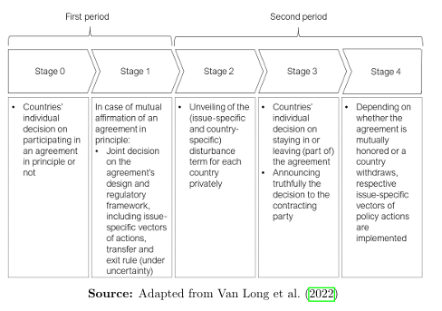
demonstrates the process of the game. The game starts by the countries’ decision as to whether they are willing to join an agreement in principle. Agreeing to that is a requirement for further international cooperation. Furthermore, incorporating an agreement in principle ensures that both countries conduct the most adequate policy actions in response to its own and its counterpart’s decision. As already stated, uncertainty comes into play when looking at cooperative out-comes. A key assumption in this setup is that negotiations on planned activities and transfer payments as well as the exit rule are conducted under uncertainty (in period one), hence, before the realisations occur (in period two). In this regard, the predetermined exit rule (period one) plays a significant role. The exit rule specifies that a country cannot partially withdraw from a pooled agreement, but is obliged to end cooperation on both issues. In order to be able to withdraw from only one agreement, the countries must have previously agreed on two separate agreements (ringfencing).

The pre-set exit rule implies that agreement(s) can only be honored or quit, at conditions agreed in period one. Hence, there is no chance of adopting agreement(s) ex post (negotiation) to the actual realisations. Since the realisations are private information and thus, there is no possibility to examine a reported real isation; neither party would agree to adjust the transfer rate in favour of the other party ex post. Since reporting would be cheap talk, instead of reporting their status, both countries inform the other party of their decision to comply with or leave the agreement before any policy action is taken.

Moreover, binding negotiations preceding realisations is important as this precludes the chance of renegotiating. By allowing the exit rule to be changed to a partial exit, pooling issues would be without consequences and not differentiate from ringfencing at all. Since private information about realisations cannot be verified, a country would have an interest to report a negative aggregate payoff in order to force a partial exit- given the country experiences one bad and one good realisation. Rene gotiation is not possible.

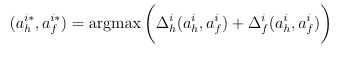
By pursuing the agreement in principle, the optimal action plan for issue i is set within the framework of the negotiations. The optimal action plan is determined by both countries (c ∈ {h,f}) such that the aggregate expected welfare gain is maximised. This is given by

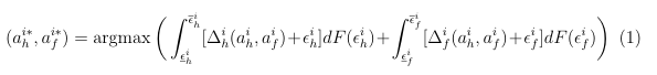
where ϵic (ϵic) denotes the smallest (largest) value of ϵi c, c ∈ {h,f}. F(ϵi c) is the cumulative distribution function of ϵi
c. Gains from cooperation of country c are defined by ∆i c(ai h,ai f), given both countries mutually consent to the action plan for issue i (ai h,ai f). Its maximum is defined by ∆i c(ai∗ h,ai∗ f).
Since the expected value of the disturbance term is zero, the maximised action plan reduces to

(2)

In this context, the optimal actions taken for both countries do not depend on the distribution of anticipated gains among countries, nor on the choice of strategy (ringfencing versus issue linkage). The latter implies that ex ante none of the strategies promises a higher gain. Van Long et al. (2022) assume that both negotiating countries display the same bargaining power. This implies that if both countries are committed to continuing the agreement, the transfer will equalise the gains from cooperation. For ringfencing, there is for each agreement an issue-specific transfer Ti∗
hf. For pooling, an issue-independent transfer T∗ hf brings the balance in gains. In the symmetric model, both countries have equivalent expected payoffs. Therefore, ex ante the transfer both countries agree on for ringfencing and issue linkage re spectively is zero. Van Long et al. (2022) further assume that the actual gains from cooperation and transfer payments can take values such that both countries mightprefer to leave the agreement for both strategies.

The baseline model does not incorporate cross-country correlation and thus focuses on an agreement being affected by idiosyncratic shocks. A shock solely directly im pacts the payoff of the country in which it occurs. A positive shock on issue i in country h implies realisation ”good” (ri h = gi h), whereas a negative shock on issue i in country h implies realisation ”bad” (ri h = bi h)- equivalent for country f. Thus, per issue per country are just two realisations possible. A good realisation occurs with probability q, where 0 < q < 1. Since realisation is binary, the probability that a country has a bad realisation is 1-q. For the case of just one issue, both countries in dependently decide on whether they want to honor or to leave the agreement. This decision takes place after both countries observe their country-specific realisation on issue i in period two.

The possible combinations of realisations are either both countries get realisation ”good” ((rh,rf) = (gh,gf)), one country gets a good realisation whereas the other one gets ”bad” ((rh,rf) = (gh,bf))/ ((rh,rf) = (bh,gf)) or both countries experience a negative (idiosyncratic) shock ((rh,rf) = (bh,bf)). If a country suffers a negative shock, rc = bc where c ∈ {h,f}, it will exit the agreement on issue i. Function π(rh,rf) assigns value G to realisation ”good” and value B to realisation ”bad”. G implies a positive payoff, whereas B provokes a negative payoff. An important assumption of the model is that ex ante, cooperation is ex pected to yield a positive payoff, implying qG + (1 − q)B > 0. Furthermore, it is assumed that a bad realisation is compensated by a good realisation, such that G+B>0. Thus, except for the case (rh,rf) = (bh,bf), it would be more profitable for both countries to commit to staying in the agreement rather than leaving it. However, if period two is characterised by non-commitment, each country focuses

exclusively on its own payoff. The agreement will only continue to exist if for both countries realisation gc occurs. In the event of a negative idiosyncratic shock, the affected country would exit the agreement. Terminating cooperation would yield a zero payoff by assumption. Thus, exit prevents the country from a negative payoff for this issue. If the partner experiences a positive shock instead, its payoff would be reduced to zero in response to the other’s exit. Accordingly, both countries would render a zero payoff. Under commitment, however, for the cases (rh,rf) = (gh,bf) and (rh,rf) = (bh,gf), the agreement would continue as G + B > 0. Social welfare maximisation would yield a higher payoff as it does under non-commitment.

In the following, two issues are considered. The analysis examines the question under which conditions countries choose ex ante a pooled agreement rather than single agreements per issue. Countries can either prefer joining a pooled agreement for both issues or they can set up one agreement for each issue i={1,2}. In the case of a pooled agreement, the exit rule set out in period one, which prohibits a partial exit and determines zero profit for both countries in case cooperation ends, applies.

It is still assumed that country-specific realisations on issue i are independently distributed, thus uncorrelated. Furthermore, assumption is made that success prob abilities of good, respectively bad realisations do not vary across issues as well as across countries (q1 = q2 = q, respectively (1 − q1) = (1 − q2) = (1 − q)). Good and bad realisations across issues, by contrast, yield different outcomes (G1= G2 and B1= B2). In order to determine which strategy is more advantageous, the expected payoffs of issue linkage and ringfencing must be compared with each other. In general, conditional on the partner to honor the agreement, the expected payoff of a country from entering an agreement is calculated by the weighted average of all possible outcomes. Thereby, the ex ante probabilities of this country are considered.

Similar to the case with one issue, we assume qGi+(1−q)Bi and Gi+Bi > 0. The expected value of cooperation on issue i is positive. Moreover, a bad realisation on issue i can be more than compensated by a good realisation of the partner on the same issue. This makes cooperation on this issue mutually desirable.

In case of ringfencing, country c stays in the agreement on issue i if and only if its respective realisation is Gi. As mentioned before, this is materialised by probability q. Thus, country c exits an agreement if Bi is realised. The country’s payoff is then normalised to zero. This yields an expected gain from ringfencing by qGi. Since the expected payoff for country c is conditional on the probability that the partner remains in the agreement(s), the expected gain needs to be multiplied by q. Hence, the expected payoff under ringfencing for both issues reads

 

E(Vring) = q2(G1 +G2)

When it comes to issue linkage instead, country c stays in the agreement as long as its expected payoff of both issues combined is positive. For this to occur, country c experiences two good realisations or the positive outcome of one issue must overcompensate for the negative outcome of the other issue. The most optimistic scenario for issue linkage is that as soon as a country gets one good outcome for an issue i, its payoff will be positive: G1 + B2 > 0 as well as G2 + B1 > 0. For this configuration (configuration 1), country c will stay in the agreement if the combi nations of realisations leading to the following outcomes are materialised: G1 + G2 with probability q2, G1 + B2 with probability q(1 − q), B1 + G2 with probability (1 −q)q. Under configuration 1, country c stops its cooperation within the scope of the pooled agreement if and only if B1+B2 is realised. This occurs with probability (1 − q)2 and yields zero payoff for both issues. The probability that the partner continues cooperating is, therefore, 1 − (1 − q)2. By applying the second binomial formula, this term can be simplified to q(2 − q). The following equation denotes the expected gain from joining a pooled agreement under configuration 1, given the partner honors the agreement (therefore multiplied by q(2 − q)).

E1(V pool) = q(2 − q)[q2(G1 + G2) +q(1 −q)(G1 +B2)+(1−q)q(B1 +G2)]

where the subscript of E denotes the type of configuration, i.e. subscript 1 stands for configuration 1. Simplifying yields

E1(V pool) = q2(2 − q)[G1 + G2 +(1−q)B1 +(1−q)B2]

(4)

By comparing the expected payoffs resulting from issue linkage, given G1 + B2 > 0 (condition 1) and B1 + G2 > 0 (condition 2), and ringfencing, a third necessary condition for pooling to dominate ringfencing can be established.

E1(V pool) = q2(2 − q)[G1 + G2 +(1−q)B1 +(1−q)B2] > E(Vring) = q2(G1 +G2)

Simplifying yields condition 3:

(G1 +G2)+(2−q)(B1 +B2) > 0

(5)

As already mentioned, the two conditions G1+B2 > 0 and B1+G2 > 0 are necessary for pooling to dominate, i.e configuration 1 needs to hold. This results from the fact that under the other two configurations covered by the model, the respective expected payoff from issue linkage is smaller than that of ringfencing. This is shown in the following. Configuration 2 is defined by G1 + B2 > 0 and G2 + B1 < 0, in other words, a bad realisation in issue 2 can be more than compensated by a good realisation in issue 1. A bad realisation in issue 1, on the other hand, cannot be counterbalanced. In such a case, the country concerned decides against cooperation. Configuration 3 is the counterpart to configuration 2 and thus defined by G1+B2 < 0 as well as G2 +B1 > 0. Having said that a country will exit the pooled agreement under configuration 2 in the case of having a bad realisation on issue 1, the exit probability (also for the partner) is given by (1-q). This means that the probability for a country of remaining in the agreement, equals q. Hence, the expected gain for a country from joining a pooled agreement under configuration 2 is the following:

E2(V pool) = q[q2(G1 + G2) + q(1 −q)(G1 +B2)] = q2[G1 +qG2 +(1−q)B2]

Subtracting E(V ring) from E2(V pool) and simplifying yields a negative result imply ing that E2(V pool) < E(V ring):

E2(V pool) − E(V ring) = q2[G1 + qG2 +(1−q)B2]−q2(G1 +G2)
=G2(q3 −q2)+B2(q2 −q3) < 0

where G2 > 0, B2 < 0 and q3 < q2. The same approach and reasoning applies, suggesting that the expected payoff from pooling in configuration 3, E3(V pool) is  also less than the payoff after ringfencing, E(V ring):

q[q2(G1 + G2) +(1−q)q(B1 +G2)] = q2[G2 +[qG1 +(1−q)B1]] < q2(G1 +G2)

The intuition behind the result that the three conditions must be satisfied for the expected payoff of issue linkage to dominate over ringfencing is illustrated by the following example: Suppose country h has realisation ”bad” in issue 1 and realisation ”good” in issue 2, whereas country f gets a good realisation in both issues. Under ringfencing, a country c exits if it has a bad realisation in an issue. In this example, country h would leave agreement for issue 1. However, this implies a zero payoff for both countries for issue 1. This in turn implies a negative externality of country h’s decision on country f for issue 1 since it has a good realisation.

Given pooling, the exit of a country under ringfencing can be prevented, since a bad realisation in one issue is overcompensated by a good one in the other issue. This is what conditions 1 and 2 represent. In this case, country h would not exit since B1 + G2 > 0. The negative externality that can occur under ringfencing is eliminated under pooling. However, the bad realisation in issue 1 affects the payoff negatively, so that country h suffers a loss in a pooled agreement compared to ringfencing, since G1 > G1+B2.

Circumventing the exit in ringfencing by entering into a pooled agreement would only be reasonable and socially desirable as long as the (expected) loss country c accepts under pooling would not outweigh the (expected) externality that a withdrawal from the single agreement under ringfencing would have for the partner. Hence, issue linkage would prove to be the preferable strategy in the case described as G1 >−B1 holds.

Note that these considerations take place ex ante, so realisations are not yet known. If these three conditions are fulfilled, it is reasonable ex ante to enter into a pooled agreement and to hedge against the occurrence of possible negative externalities.

4 Extension

This section aims to clarify the implications of common shocks on expected payoffs of issues treated separately compared to expected payoffs of pooled issues. Com pared to Van Long et al. (2022), the innovation of the section is the introduction of common shocks. In this context, it examines whether one of these two strategies relatively dominates ex ante the other when common shocks are considered. To investigate this, the agreements under consideration are no longer subject to idiosyncratic shocks but to common shocks. Common shocks imply a positive cross-country, inner-issue correlation of the realisations. Compared to the case of uncorrelated re alisations, this induces a higher probability that both countries h and f experience the same realisation for issue i. This naturally applies to both positive and negative realisations. Here, it is illustrated using the case of positive shocks:

P(rih = Gi andrif = Gi) > P(rih = Gi)∗P(rif = Gi)

The following table (Table 1) illustrates the change in joint probabilities of possible outcome combinations by the introduced correlation. It is important to emphasise that the underlying analysis is carried out following the baseline model under the assumption that the success probabilities of good and consequently also bad reali sations are identical across issues, in other words qi = q and (1−qi) = (1−q). The positive cross-country correlation parameter is denoted by z. While the probabilities of both countries experiencing an equal shock for the same issue increase by factor z to q2 + z (positive shock) and (1 − q)2 + z (negative shock), the probabilities of non-aligned realisations for the same issue decrease by factor z to q(1 − q) − z. This methodology allows an increase in z to reflect a rise in the covariance. z must, thereby, lie in between zero and q(1−q).

Note that for z equals zero, the realisations are iid which is covered by the baseline model. The upper limit results from the fact that a probability cannot take a negative value. z can take the realisations x and y, where x denotes the correlation parameter for the cross-country realisations on issue 1 and y respectively the correlation parameter for the realisations on issue

2.

A ringfenced agreement for issue i will just continue if both countries experience
Table 1: Joint probability matrix for calculating expected ringfenced payof

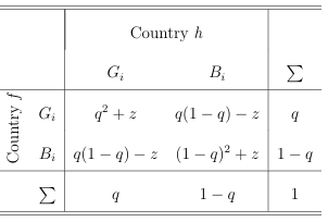
Note: z ∈ {x,y} where 0 < z < q(1−q), i ∈ {1,2}

x (y) is the correlation parameter for the cross-country realisations on issue 1 (2). The success probability of a good realisation is q, of a bad realisation (1 − q) respectively, where 0 < q < 1. Gi denotes an issue-specific outcome of a good realisation, whereas Bi defines an issue-specific outcome of a bad realisation. Source: Own illustration

a positive shock for issue i. This is materialised with probability P(ri h = Gi and

ri f = Gi) = q2 +z and yields outcome Gi for each country (see Table 1). Note, the probability of getting a good realisation in issue i for country c is unaffected by the imposed correlation. Hence, country c continues cooperation for issue i with proba bility q (see Table 1). From a country’s perspective, its exit probability remains the same, but the overall exit probability falls compared to the baseline case. The latter can be explained by an increase in the counter probability: the success probability of both countries experiencing a good realisation in issue i is no longer q2, but now q2 +x. Each country now anticipates that, first, it will continue to cooperate under ringfencing with probability q and, second, if it experiences a good realisation on issue i, the probability increases so its partner will also experience a positive shock on this issue3. In this section, we assume configuration 1 to hold. Hence, cooperation occurs in pooling as long as a country c does not experience a negative shock in both issues. The exit probability is thus determined as follows:

 

P(r1 c = B 1 and r 2 c = B 2) = P(r 1 c = B 1)∗P(r 2 c = B 2) = (1−q)2

 

The probability that country c will cooperate is its counter probability 1−(1−q)2 = q(2 −q). This probability remains also unaffected by the introduction of a positive inner-issue correlation across countries. Although the exit probability of a country stays the same, for the following procedure it is not relevant. Since joint probabilities reflect how likely constellations with both countries having a certain realisation are

3 Note that cross-issue correlation is still not assumed. Hence, these probabilities
remain unaffected by the innovation.

observed, the overall exit probability and its respective counter probability matter. But from the beginning: the approach to calculate the expected pooling payoff fol lows the same logic as in the case without correlation (see Section 3). The expected payoff is calculated both times for and from the perspective of one country. The possible combinations of outcomes for both issues are multiplied by their respective probability of occurrence, conditional on that the partner remains in the agreement. Opposing to the case in Section 3, however, the joint probabilities related to an issue i change due to the inclusion of correlation (see Table 1).

Table 2 shows all the combinations of joint probabilities relevant for calculating the expected payoff for the countries h and f on the issues 1 and 2. In the following, the structure of Table 2 is explained by means of the first cell: The first (second) term of the first cell denotes the joint probability for both countries to experience a positive shock on issue 1 (2). This leads to an outcome G1 (G2) for each country. The probability of both countries experiencing positive shocks on each of their issues is simply the product of the two joint probabilities.

Even though the exit probability of one country remains unaffected, we cannot simply multiply the expected payoff by its counter probability. This is due to the fact that correlation affects probabilities differently, more precisely depending on the partner’s realisations. For each pair of realisations from a country yielding a certain outcome, there are three possible pairs of realisations for which the partner country stays in the agreement. For instance, country h generates outcome combination
(G1,G2) through realisations (r1 h = g1 h,r2 h = g2 h). For this outcome pair, country f could potentially have one of the following three output pairs: (G1,G2), (G1,B2) or (B1,G2). Depending on the partner’s combination, a different joint probability

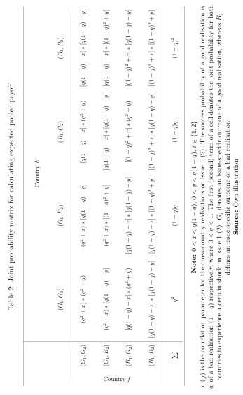
results. This is due to correlation affecting non-aligned cross-country realisations negatively and aligned cross-country realisations positively. Note that the fourth row and the fourth column are irrelevant for the calculation of the payoffs, since in these combinations the country whose realisations are both bad quits cooperation. The payoffs for both countries are then normalised to zero as before. The combi nations of realisations where both countries stay in the pooled agreement are thus, expressed by the 3×3 matrix.

After the basic framework is established, the influence of correlation on the relative expected payoffs of ringfencing and pooling is determined first at the simplest case, the symmetric case. The symmetric case is defined by identical success probabilities across issues, in other words, qi = q and (1 − qi) = (1 − q). Furthermore, the outcomes across issues do not differ from each other, saying Gi = G and Bi = B. Both issues are positively correlated to the same degree implying x = y > 0. Since x equals y, y is replaced by x in the following analysis. We show that the following results hold for the symmetric case:

Lemma 1

If qi =q, Gi =G respectively Bi = B, G+B > 0, qG+(1−q)B > 0 and x = y > 0, the partial derivatives of the expected payoffs with respect to the correlation parameter x (y) have a positive sign. This implies that the expected payoffs of ringfencing and issue linkage increase in x (y).

The proof below derives Lemma 1 and Proposition 1. In this context, Lemma 1 forms the foundation for the proof of Proposition 1 and steps are intertwined.

Proposition 1

If qi = q, Gi = G respectively Bi = B, G+B > 0, qG+(1−q)B > 0 and x = y > 0, issue linkage becomes ex ante relatively less attractive compared to ringfencing since the expected payoff from ringfencing increases relatively to a greater extent with x (y) than the expected payoff from issue linkage.

Proof.

In order to prove the above results, we start from calculating the expected payoff from ringfencing two issues. For ringfencing, the approach to the calculation is exactly the same as in Section 3. As already explained, a country c will exit agreement on issue i if its realisation in the respective issue i turns out to be bad. Thus, the agreement on issue i is just continued by both countries if and only if (ri h, ri f) = (gi h, gi f). Since the success probabilities across issues and the issue-specific correlation parameters do not differ from each other, P(r1 h = G and r1 f = G) equals P(r2 h = G and r2 f = G). With G1 = G2 = Grespectively B1 = B2 = B, the following expected payoff from two separate agreements is

E(˜ Vring xy ) =2G∗P(ri h = Gandri f = G) = 2G∗(q2 +x)

where x = y > 0 is formally expressed by subscript xy and E(˜ V) denotes the expected payoff for identical outcomes across issues. We consider country h for the calculation of the expected payoff from entering a pooled agreement4. Since cross-country correlation is considered, the expected payoff cannot be multiplied by the exit probability of the partner. To account for the fact that there are three different probabilities of obtaining a specific outcome combination depending on the realisations of the partners, the expected value from pooling in the symmetric case is calculated as follows: The probability that country h realises 2G is computed by summing up the first three cells of the first column of Table 2: (q2 + x)2 + (q2 + 4 Since countries are symmetric, the results do not differ between countries.

x)((1−q)q−x)+((1−q)q−x)(q2+x). Furthermore, country h realises (G+B) with probability [(q2 +x)((1−q)q −x)+(q2 +x)((1−q)2+x)+((1−q)q−x)2]∗2 (sum of the joint probabilities of the first three cells of the second and third column each) since we do not differentiate between outcomes across issues in this case. Taken together and simplified, with G1 = G2 = G respectively B1 = B2 = B, this results in the following expected gain from joining into a pooled agreement:

E1(˜ Vpool xy ) =2(2−q)q2(G+B(1−q))+2(1−q)(G+B(1−2q))x+2Bx2

In order to compare the magnitude of the marginal effect on expected payoffs caused by common shocks, partial derivatives as a function of the correlation parameter must be computed first. The partial derivative of the expected payoff under ringfencing with respect to x is given by

∂E(˜ Vring xy )by ∂x =2G

(6)

Partial differentiation of the expected payoff from pooling with respect to x yields

∂E1(˜ Vpool xy )by∂x =2(1−q)(B +G−2Bq)+4Bx:=f(q)

(7)

Note that both derivatives are positive. In the case of ringfencing, it is straightfor ward to see that the relative change in expected terms is greater than zero since G is a positive real number. We have relegated the details of explaining the positive sign of the partial derivative of the expected payoff from issue linkage to Appendix A.1. This proves Lemma 1. Intuitively, the result is interpreted to indicate that the expected payoffs for both ringfencing and issue linkage increase with x5. The rise in expected payoffs can be attributed to the fact that cooperation between the two countries becomes more likely regardless of the type of agreement. As already explained, the overall probability of cooperation under ringfencing and inclusion of correlation increases to q2+x. For issue linkage, the probability that both countries honor the agreement is calculated by adding up the nine probabilities of the 3×3 matrix. For x = y > 0, this overall probability for cooperation (already simplified) is given by

2x +((−2+q)q +x)2

(8)

If we set x in equation 8 equal to zero, then the term simplifies to ((−2 + q)q)2. In this case, the extended model reduces to the baseline model of Section 3. Since Van Long et al. (2022) determine the probability that a country c remains in the agreement to be q(2 − q) under configuration 1, the joint probability that both countries continue in the agreement is thus q(2 − q)q(2 − q) = ((−2 + q)q)2. Thus, this is consistent with the probability we calculated. Equation 8 increases in x since the sign of its partial derivative with respect to x is positive, for all values of q:

2((−1 +q)2 +x) > 0

Hence, we can conclude that the result indicates that bilateral cooperation becomes more likely regardless of the agreement when positive cross-country, inner-issue cor relation is taken into account.
Having clarified that correlation causes expected payoffs to increase (Lemma 1),
5 Due to symmetry, the same holds if we conduct the analysis with y instead of x.

we now examine which expected payoff rises to a greater extent in relative terms (Proposition 1). The details of comparing the magnitudes from equation 6 with equation 7 are relegated to Appendix A.2. The appendix shows that in the symmetric case, an increase in the correlation parameter x induces a rise the expected payoff of ringfencing relatively more than the one of issue linkage. Similar to the proof of Lemma 1, the insights for x can be replicated for y. The occurrence of common shocks relatively favours the strategy of ringfencing. This finalises the proof of Proposition 1.

The intuition behind this result of Proposition 1 can be explained by looking at the scenarios of the 3×3 matrix in a differentiated manner. Note that the scenario where both countries get good realisations for both issues is equally included in the cal culation of expected values, irrespective of the strategy considered. Therefore, this scenario cannot be crucial for the discrepancy in marginal effects between ringfencing and pooling. However, in contrast to ringfencing, under configuration 1 another eight constellations are possible, under which both participating countries continue the pooled agreement.

Consider first the scenarios characterised by non-aligned realisations of both countries on both issues. These yield the following outcome pairs: (i) (B,G) for country h and (G,B) for country f and (ii) (G,B) for country h and (B,G) for country f. If these scenarios occur, a pooled agreement would be favourable compared to two single agreements. This is due to the fact that under ringfencing each country would withdraw from the agreement covering the issue at which its realisation is bad. This would have the consequence that each country’s exit in the respective issue would cause a negative externality for the partner. The negative externality results from the fact that the partner country could have made a positive gain due to its good implementation on this issue. With the exit of the counterpart, however, the gain for this issue declines to zero. In sum, no agreement would continue. The total payoff for both countries would be zero. Pooling, instead, would yield a positive gain for both countries since G + B > 0. This proves that pooling is the advantageous strategy if one of these scenarios were to happen. However, the introduced correlation reduces the likelihood for these scenarios to occur.

This can be seen by taking a look at the probability of occurrence [q(1 − q) − x]2 (see Table 2). The effect of x on this probability is unambiguous. Both factors diminish by factor x each. This in turn causes the product to decrease. The overall effect of scenarios (i) and (ii), favouring issue linkage but becoming less probable, is evidence supporting
the result from Proposition 1. Consider second the scenarios in which the realisations of both countries on both
issues are aligned, yielding the following outcome pairs: (iii) (G,B) for country h and (G,B) for country f and (iv) (B,G) for country h and (B,G) for country f.

If one of these constellations is realised, having earlier signed two single agreements is better than having agreed to one pooled agreement. The rationale for this is that under ringfencing both of the countries would eliminate the agreement of that issue where both have a bad realisation. This, in turn, stems from the fact that this issue implies a negative outcome. This improvement due to a partial exit, however, would not be possible under pooling. Hence, the payoff for both countries would be moderated by cooperating still on the issue as part of the pooled agreement where a negative common shock has occurred. For these scenarios, correlation increases the likelihood of occurrence. As already shown in Table 2, for these cases the probability increases by factor x each to (q2 + x)[(1 − q)2 + x] for scenario (iii) and to [(1 − q)2 + x](q2 + x) for (iv). The overall effect of these two scenarios, favouring ringfencing and becoming more likely, is further evidence in favour of the result from Proposition 1.

Third, we scrutinise the scenarios characterised by non-aligned realisations on one issue and aligned realisations on the other issue across countries, yielding the following outcome pairs: (v) (G,G) for country h and (G,B) for country f, (vi) (G,G) for country h and (B,G) for country f, (vii) (G,B) for country h and (G,G) for country f and (viii) (B,G) for country h and (G,G) for country f. If one of these scenarios occurs, pooling the two issues is preferable to ringfencing two agreements. The rationale is explained vicariously by scenario (v). Since G + B > 0 holds, country f would stay in the pooled agreement and would not trigger a negative externality for country h.

Symmetry implies that the outcome from a good realisation on issue 2 for country h is also larger than the absolute value of the outcome from a bad realisation on issue 2 for country f. Hence, symmetry means the (expected) negative
externality for country h is larger than the (expected) loss country f would experi ence when exiting the pooled agreement. This makes issue linkage jointly desirable for these scenarios.

To determine how these scenarios contribute to the explanation of Proposition 1, we need to find out whether these scenarios underpinning issue linkage become more or less likely with the introduction of correlation. Given x = y and q1 = q2 = q, these four scenarios occur with the same probability, which is given by (q2+x)[q(1−q)−x]. Unlike the previous scenarios, it is not unequivocal to see how the probabilities be have as a function of x. This is due to the fact that correlation induces countervailing effects. Irrespective of the issue, correlation strengthens the joint probability of the vent (ri 2h = gi h,ri f = gi f) and weakens the joint probability for (ri h = gi h,ri f = bi f) and (ri h = bi h, ri f = gi f). In order to better clarify the role of correlation, the probability (q2 + x)[q(1 − q) − x] is partially derived with respect to x. The partial derivative, which is q−2q2−2x, reveals that the change in probabilities of the four scenarios due to the change with x depends crucially on the success probability q. For x = 0, the derivative is positive when q < 0.5 and becomes negative once q > 0.5. If q < 0.5, G needs to be correspondingly large in order to meet condition qG +(1 −q)B > 0. It follows that G, the outcome of a good realisation must be relatively high, however, the probability of this to occur is low. If q > 0.5, then G need not necessarily take a value higher in absolute value than B for qG + (1 − q)B > 0 to hold. However, this would violate condition G + B > 0. Hence, the binding constraint for the case where q > 0.5 is G+B > 0.

When introducing correlation for all defined values (0 < x < q(1 − q)), the par tial derivative for q > 0.5 is even smaller than without correlation since −2x < 0. This can also be explained intuitively. As already mentioned, on the one hand, the marginal effect of x on the issue for which the cross-country realisations are both good is positive. This marginal effect of x is small relatively to the high success probability q > 0.5. On the other hand, the same marginal effect of x on the issue for which the cross-country realisations are non-aligned is negative and relatively strong with a high success probability. In aggregate, the effect on probability is neg ative. This implies that these four scenarios get less likely for q > 0.5. Since these scenarios favour issue linkage, this overall effect is in line with the other scenarios characterised by crossed respectively aligned (cross-country) realisations.

Conversely, for a low success probability q < 0.5, and a small x, more precisely x < 1 2 (q − 2q2), the effect on probability becomes positive. On the one hand, a marginal increase in x enhances the initially relatively low probability of both countries experiencing a positive shock on one issue. On the other hand, a marginal effect of x of the same factor reduces the relatively high probability of non-aligned realisations on the other issue relatively less.

Therefore, given a small success probability and a small x, the four scenarios favouring issue linkage become more probable by a common shock. Correlation has an overall strengthening effect on the expected payoff from pooling two issues here. Concluding, the marginal effect of x on probability is positive for q < 0.5 respectively small x and negative for q > 0.5. Hence, without knowing the exact value for q, we cannot determine whether these four scenarios become more or less likely through common shocks. What we can state with certainty, however, is that at first all overall effects reflect the result of Proposition 1 given q > 0.5 holds.

Secondly, the overall effect of these four scenarios for q < 0.5 and a small x (making issue link age relatively more likely) counteracts the other overall effects (making ringfencing relatively more likely) but cannot overcompensate for them. This is due to the fact that for the symmetric case, ringfencing relatively dominates over issue linkage as results indicate.

Overall, results indicate that in the event of common shocks, each participating country should therefore anticipate ex ante that the scenarios in which it suffers a loss under pooling relative to ringfencing will occur more frequently. At the same time, it is less likely that those situations will occur where pooling prevents negative externalities and the termination of single agreements.

The result of Proposition 1 can be generalised in various manners. These are sum marised in Proposition 2.

Proposition 2 .

Suppose qi = q, G1= G2 respectively B1= B2, Gi+Bj > 0 (with i= j and j ∈{1,2}) and x = y > 0. If Gi+Bi > 0 and qGi+(1−q)Bi > 0, issue linkage becomes ex ante relatively less attractive than ringfencing with an increase in correlation parameters. This result extends to the case (given B1 = B2), where the assumption of x = y > 0 is replaced by non-equal correlation parameters- namely x >0 and y =0 and vice versa.

Proof.

In order to prove Proposition 2, we now scrutinise two further cases as part of our extension. Like the symmetric case, they are defined by a common q but differ from the symmetric case in terms of the outcomes across issues. Now, the same realisation yields issue-specific outcomes Gi and Bi, meaning G1= G2 and B1=B2. The second application distinguishes itself from the first by modified correlation parameters x and y. Within the first case, both correlation parameters are considered to be positive, i.e. x = y > 0. In the second case, x and y do not take the
same value. Issue 1 is positively correlated implying x > 0, whereas issue 2 remains uncorrelated, indicating y = 06. Since the general approach does not differ from the symmetric case, we have relegated the discussion of these cases to Appendices B.1 and B.2.

In Appendix B.1, we analyse issue-specific outcomes instead of symmetric outcomes across all issues, all other things being equal to the case before. We show that the
6 In order to prove that Proposition 2 holds for the second application, in this application, we impose assumption B1 = B2 to get a mathematical solution.

expected payoff from ringfencing also rises relatively more in x than that from issue linkage. As a matter of intuition, this result can be derived in the same way. When compared to the symmetric case, none of the probabilities change because they do not depend on the level of outcome. Also, the scenarios characterised by non-aligned respectively aligned (cross-country) realisations are unaffected by the innovation. This is firstly explained by constant probabilities. Secondly, since configuration 1 is still considered, implying G1 +B2 > 0 and B1+G2 > 0 respectively, there is also no change that pooling would be the preferred strategy in case of scenarios (i’) 7 and
(ii’) and ringfencing respectively for scenarios (iii’) and (iv’). For scenarios (v’) to (viii’), which are characterised by non-aligned realisations on one issue and aligned realisations on the other issue across countries, symmetry cannot be assumed for different issue-specific outcomes. Hence, Gi +Bj > 0 no longer implies Gi +Bi > 0.

However, the latter is imposed by assumption. Therefore, regarding these scenarios, issue linkage would be preferable to ringfencing since Gi > −Bi holds. Remember that it is uncertain if scenarios (v’) through (viii’) are rendered more or less likely by a common shock. The inference remains unchanged compared to the symmetric case. In these scenarios, if q < 0.5 and x is small, issue linkage would get more likely. Hence, this overall effect of the common shock would contradict the overall effects of scenarios (i’) to (iv’). As shown in the intuition of Proposition
1, the opposite is true for q > 0.5. Concluding, even if the overall effect would be that scenarios (v’) to (viii’) which foster issue linkage become more likely, it would remain weaker than the other overall effects that make ringfencing relatively more
7 (i’) denotes scenario (i), the only difference being that asymmetric outcomes apply in (i’). The same manner of designation also applies to scenarios (ii’) to (viii’) likely.

Having shown that different outcomes across issues have no influence on the result of Proposition 1, we now analyse the effect of modifying the correlation parameters. In B.2, we derive the results for the case framing that x and y are non-equal. We find that setting one correlation parameter to zero (and additionally imposing B1 = B2) does also not change the fact that the expected payoff from ringfencing rises relatively more than the expected payoff from issue linkage when cross-country correlation increases. Again, the intuition behind the results is fundamentally the same.

When reviewing the scenarios characterised by non-aligned realisations of both countries in both issues, we see that correlation lowers the probability of these occurring to [q(1 − q) − x][q(1 − q)] compared to no cross-country correlation (x=0). Mathematically, the correlation leads to a reduction of the first factor, which diminishes the product. The effect on probability is consistent with the scenarios of the cases where x = y > 0 holds. However, this effect is weaker compared to the scenarios conducted under x = y > 0, since [q(1 − q) − x]2 < [q(1 − q) − x][q(1 − q)]. This implies relative to the cases for x = y > 0 that these scenarios occur when x > 0 and y = 0 holds, more frequently. However, for scenarios in which the realisations of both countries on both issues are aligned, correlation boosts the probabilities rel ative to no cross-country correlation at all. For the scenario where both countries have a positive common shock in issue 1 (2) and a bad realisation on issue 2 (1), each is enhanced to (q2 + x)(1 − q)2 respectively [(1 − q)2 + x]q2. In comparison to the symmetric case, the effect on probabilities is not as pronounced in these two scenarios since just the joint probability of both countries experiencing a common shock on issue 1 is affected positively by correlation.

Remember that for scenarios in which only one of the two countries suffers from a bad realisation in one issue and otherwise only good realisations occur, the change in probability cannot be clearly determined for the cases with x = y > 0. The rationale is that correlation causes countervailing effects and depends decisively on q. In the case considered here, we can unambiguously specify the effect on probability for each scenario separately since just the first factor changes by correlation. The probabilities of the two scenarios in which the realisations of both countries in issue 1 are non-aligned diminish as x increases, holding q constant. The probabilities of the other two scenarios in which both countries experience a positive shock in issue 1 increase in x. This becomes apparent in each case from their partial derivatives with respect to x, which is −q2 < 0 for the first two scenarios and q(1−q) > 0 for the latter.

Therefore, between scenarios there are still countervailing effects on probability. The dominant effect critically depends on q. For q < 0.5, | q(1 − q) |>| −q2 | implying that the cumulative effect on probability of these four scenarios is positive. For q > 0.5, however, the cumulative effect on probability is negative. Remember compared to the symmetric case, the effects on probabilities for the scenarios characterised by non-aligned realisations of both countries in both issues respectively aligned realisations of both countries in both issues, each go in the same direction, but are not as strong as in the symmetric case. As already explained, under configuration 1, issue-specific outcomes (for good realisations) do not change the fact that pooling would be the preferred strategy for the former scenarios, whereas ringfencing respectively for the latter. The case considered here (Gi and B1 = B2 = B) is a symbiosis of symmetric and asymmetric (issue-specific)

outcomes. The insights for these outcomes do not change for this case because conditions convert to G1 + B > 0 and G2 +B > 0. As in the symmetric case for the scenarios characterised by non-aligned realisations on one issue and aligned realisations on the other issue across countries, it is also uncertain how the probability changes with x. Given the assumption that B1 = B2, for these four scenarios, it can as well be determined that issue linkage is ex ante jointly more desirable. Looking at the results, we can say that regardless of which case occurs, the overall effect of these scenarios, no matter how it transpires, do not outweigh the overall effects of the other scenarios. Hence, we can conclude that the direction of the total effect is the same to that of the symmetric case.

Following the same approach as before, we are not able to prove mathematically that issue linkage is preferred to ringfencing in the case of x > 0 and y = 0 as well as B1= B2. The simplifying assumption B1 = B2 = B allows us to generalize results from Proposition 1. Implications of dropping assumption are left for future research.
□
Lastly, we point out that the entire analysis was conducted under configuration 1 is not a restrictive assumption. The robustness of the results under configuration 1 confirms that there is no necessity to examine more pessimistic scenarios for issue linkage such as under configuration 2 and 3. This can be illustrated using the results of the baseline model (Section 3) where it was shown that for issue linkage to be the preferable strategy per se, Gi + Bj > 0 needs to be satisfied. This, however, is not the case in configuration 2 and 3 (Van Long et al., 2022).

5 Discussion and conclusion

This paper has contributed to the explanation of why issue linkage is not prevalent when it comes to closing international agreements. Following the model of Van Long et al. (2022), we have conducted our analysis under uncertainty concerning actual payoffs from cooperation and by excluding partial exit regarding a pooled agree ment. In detail, our paper addressed the extent to which common shocks influence the choice between pooling issues in one agreement or treating them separately in different agreements. We conclude that the emergence of common shocks positively impacts the expected payoff of issue linkage. Although conducted under the most optimistic case for issue-linkage, our analysis highlights that issue linkage becomes ex ante relatively less attractive compared to ringfencing8 if common shocks occur.

The conditional attractiveness of issue linkage found by Van Long et al. (2022) therefore reduces with the introduction of common shocks- relative to ringfencing. Hence, given issue linkage was welfare dominant before the introduction of common shocks, such shocks might lead to issue linkage being inferior to ringfencing (ex ante). Following the original paper, it is reasonable to assume that q1 = q2 = q holds. However, one can also imagine scenarios where this is not the case. We thereupon pose the following thought experiment: What would we expect to happen in the symmetric case9 if we relax the condition that the probability of success across ex

8 In the three cases considered, the proof of the last case is conditional on symmetric negative outcomes.
9 Remember, the symmetric case is characterised by identical outcomes across is sues, saying Gi = G and Bi = B, and positive identical correlation parameters.

penditures is the same? This causes a change in the (joint) probabilities. Suppose qidenotes the success probability of outcome G occurring for issue i. First, when con sidering the scenarios characterised by non-aligned realisations in both issues across countries, we see that these scenarios loose their relative importance with x. This is due to the fact that its probability diminishes to [q1(1−q1)−x][q2(1−q2 2)−x]. Issue linkage would be the more profitable strategy if any of these scenarios occurred, but they become less likely. Thus, this overall effect is consistent with the result from Proposition 1.

Second, consider the scenario in which a positive common shock occurs on issue 1 (issue 2) and a negative common shock on issue 2 (issue 1). The probability changes to (q2 1 + x)[(1 − q2)2 + x] and [(1 − q1)2 + x](q2 2 + x) respectively.

This infers that a marginal increase in x unambiguously raises the probability, just as for the sym metric case. Since these scenarios would favour ringfencing, the overall effect of x for these scenarios is also in line with our result from Proposition 1.

Finally, consider the four scenarios characterised by a positive common shock on one issue and non-aligned realisations on the other issue. First of all, remember that these scenarios would favour issue linkage. Note that in this case the four scenarios do not all share the same probability. This is due to the fact that it makes a difference in which issue the common shock occurs because of q1= q2. Thus, the probability for the two scenarios with a positive common shock in issue 1 is (q2 1 + x)[q2(1 − q2) − x]. In contrast, the probability for the two scenarios with a positive common shock in issue 2 equals [q1(1 − q1) − x](q2 2 + x).

To what extent the probabilities change with x can be analysed by considering the partial derivative with respect to x. The partial derivative of the scenario where both countries in issue 1 experience the positive shock is −2x−q2
1 +q2−q2 2. It is noticeable that for x = 0, the partial derivative is negative as soon as q1 > 0.5. This is because from this value on, q2
1 is larger than the maximum of q2 −q2
2. The partial derivative of the scenario
in which both countries experience the positive shock in issue 2 is −2x−q2 2+q1−q2 1.

For this partial derivative to be negative at x=0, q2 must be larger than 0.5. To avoid contradictions, however, it must hold that both success probabilities q1 as well as q2 are greater than 0.5. Under this condition, the marginal effect of x on both probabilities (for all four scenarios) is negative. This is true regardless of what value x takes. Note that this result is in accordance with the symmetric case, where the probability of success q is not issue dependent. Consequently, it should not matter whether the probabilities of success in the different issues are the same or non-equal, as long as they are both sufficiently large.

The concordance of the result between the symmetric case with a common q and the case with issue-specific success prob abilities q1 and q2 is not surprising. Intuition remains the same as in Section 4.

Given high probabilities of success, a marginal increase in x affects the probability of the issue in which the positive common shock happens relatively less (positively) than (negatively) the probability on the issue whose cross-country realisations are non-aligned. Hence, in total, the probability decreases. This would make these four scenarios favouring issue linkage less likely given q1 and q2 being greater than 0.5.

With correlation, all overall effects of the varying scenarios consist of either favouring ringfencing and becoming more likely or favouring issue linkage but decreasing in their relative weight, issue linkage looses its relative attractiveness ex ante. Summing up, regardless of a common probability q or different ones q1 and q2, we expect the same outcome as long as they are larger than 0.5. The proper analysis is left to  future research.

We conclude by highlighting two further potential avenues of research. One is that our analysis in Section 4 could be further enriched by looking at agreements having at least three countries as treaty parties. In this case, two settings would be conceiv able. Firstly, it could still be considered that the agreement, irrespective of whether it is a ringfenced or pooled agreement, is terminated as soon as one country exits. Total payoffs from issue linkage would then reduce to zero for all three countries, whereas this is not necessarily the case for ringfencing. Secondly, it should be considered incorporating the eventuality that pooled multilateral agreements can continue to exist even if one country decides to leave the agreement after having observed its realisations.

This assumption is closer to reality, since it is legitimate within a multilateral agreement to permit a country to end its membership including its legal obligations by means of a withdrawal clause. The United Kingdom, for instance, has made use of the withdrawal clause (Article 50) of the Treaty on European Union and has thus unilaterally withdrawn from the European Union (EUR-Lex, 2021). Applied to our approach, this would imply that the pooled payoffs for the remaining member states would still be positive, instead of being set to zero. From this point of view, the research question could remain the same. Furthermore, one could additionally raise the question, in which of the two scenarios issue linkage ex ante is relatively more attractive.

In recent years, regional trade agreements have become more involved in their scope and incorporated more and more policy areas (Acharya, 2016). Therefore, the sec ond extension could be to incorporate more than two issues in agreements between two countries, either as one integrated agreement or as ringfenced agreements where

each covers one specific issue. This would imply an extra correlation parameter for cross-country realisations for the additional issue. Moreover, the additional issue would induce more potential scenario combinations. Following assumptions made in this paper, one could then assume that one good realisation overcompensates one bad realisation. Hence, the increase in possible outcome combinations, would also imply an increase in terms incorporated into the expected payoff for a pooled agree ment10. Therefore, the logic applied in this paper might still hold. The calculation of expected payoffs for issue linkage would still take into account scenarios including
bad outcomes (more so than in this paper), which are not relevant for calculating the expected payoffs from ringfencing. As already pointed out by Van Long et al. (2022), another interesting aspect to consider would be relaxing the assumption of symmetric countries. All these are topics for future research.

10 The number of outcome combinations incorporated in the expected payoff (for issue linkage) would further increase if one assumed that one good realisation overcompensates two bad realisations

References

Acharya, R. (Ed.). (2016). Regional Trade Agreements and the Multilateral Trading System. Cambridge: Cambridge University Press.

Barrett, S. (1997). “The strategy of trade sanctions in international environmental agreements”. In: Resource and Energy Economics 19.4, pp. 345–361. Deutsche Bundesbank (2020). Monthly Report- January 2020. [Online]. url: https: //www.bundesbank.de/resource/blob/822434/ecd683988de2a0783ddc9474c% 20438deda/mL/2020-01-monatsbericht-data.pdf. [Accessed 10 September 2022].

EUR-Lex (2021). Brexit: EU-UK relationship. [Online]. url: https://eur-lex. europa.eu/content/news/Brexit-UK-withdrawal-from-the-eu.html. [Accessed 17 August 2022].

Horn, H. and P.C. Mavroidis (2014). “Multilateral environmental agreements in the WTO: Silence speaks volumes”. In: International Journal of Economic Theory 10, pp. 147–165.

Lim˜ ao, N. (2005). “Trade policy, cross-border externalities and lobbies: do linked agreements enforce more cooperative outcomes?” In: Journal of International Eco nomics 67, pp. 175–199.– (2007). “Are Preferential Trade Agreements with Non-trade Objectives a Stum bling Block for Multilateral Liberalization?” In: The Review of Economic Studies 74.3, pp. 821–855.

Maggi, G. (2016). “Issue linkage”. In: Bagwell, K. and R. Staiger (Eds.). Handbook of Commercial Policy. Elsevier, pp. 513–564.

Nordhaus, W. (2015). “Climate Clubs: Overcoming Free-riding in International Cli mate Policy”. In: American Economic Review 105.4, pp. 1339–1370.

Poast, P. (2013). “Issue linkage and international cooperation: An empirical inves tigation”. In: Conflict Management and Peace Science 30.3, pp. 286–303.

Sebenius, J.K. (1983). “Negotiation arithmetic: adding and subtracting issues and parties”. In: International Organization 37.2, pp. 281–316.

Tollison, R.D. and T.D. Willett (1979). “An economic theory of mutually advanta geous issue linkages in international negotiations”. In: International Organization 33.4, pp. 425–449.

Van Long, N., M. Richardson, and F. St¨ ahler (2022). “Issue linkage versus ringfencing in international agreements”. In: The Scandinavian Journal of Economics.

World Bank (2005). Economic Growth in the 1990s: Learning from a Decade of Reform. Washington, D.C.: World Bank.

A Appendix

A.1 Proof of Lemma 1- issue linkage

To prove that equation 7 is greater than zero, the signs of the single components must be analysed and the magnitudes must be compared. To determine whether 2(1−q)(B+G−2Bq) > 0 (since B+G > 0 and B < 0)relatively predominates over 4Bx <0, equation 7 can first be rewritten as 2(1−q)(B +G)−4(1−q)qB +4Bx. Second, after factoring out, the second and third component can further be expressed as 4B(−q(1 − q) + x) and directly compared. Since q(1 − q) > x, we know that −q(1−q)+x < 0 and hence, 4B(−q(1−q)+x) > 0 (remember B < 0). Thus, the sum of the second and third components is greater than zero and as already stated the first component also takes a positive value. Consequently, the overall term has a positive sign.

A.2 Proof of Proposition 1

In the following, we compare the magnitudes of the equations 6 and 7, in order to determine whether expected payoffs of ringfencing or issue linkage rise sharper in x. A clear determination of the magnitude of equation 7 is not possible as it depends on x and q. However, it decreases in x as 4Bx < 0. Hence, in order to compare magnitude of equation 6 and 7 anyway, we start by comparing the maximum of equation 7 with equation 6 and thus, set x equal to zero in the former. Since the magnitude of the marginal change from pooling depends critically on q, the change in q needs to be analysed. The function is concave in q since f”(q)=8B, where B is a negative real number. As described above, we start by focusing on the maximum of q. This is determined by setting f’(q)=−2(G + B(3 − 4q)) equal to zero and is given at q∗ = 1 4 (3 + G B ). If equation 7 is smaller than equation 6, at this point q* with x = 0, it is smaller at any other defined value of q and x.

Starting from derived maximum, for G > −3B, the maximised q would be negative which cannot be feasible. The lower bound of q = 0 then determines the maximum (as the function is concave). The marginal change on issue linkage for x = 0 and q∗ = 0 is given by 2(B +G). Since B < 0, this proves that 2(B +G) < 2G. Hence, in this case, the maximum of equation 7 is smaller than equation 6.

However, for the maximal q to be an interior solution, 3 + G/B > 0 or G < −3B is required to hold. Substituting the maximising q into equation 7 with x = 0 gives the maximal value of f(q∗) and yields −(G−B)2 4B . In the following, we use this inter mediate result to prove by contradiction that the relative change of the expected payoff from ringfencing is larger than the one from pooling.

Proof by contradiction:

Assuming that the introduced correlation raises the expected payoff from entering a pooled agreement relatively more compared to ringfencing: 2G < −(G−B)2 4B , leads to the following inequality:

G2 +6GB+B2 >0

(A.1)

Calculating the intersection points with the abscissa and analysing the curvature behaviour shows that the function (left-hand side of A.1) is convex and between the roots at G = (−3 + 2√2)B ≈ −0.17B and G = −(3+2√2)B ≈ −5.83B in the negative range. Note that both roots are feasible as both values for G are positive. Byusing the conditions G > −B (rewritten from G+B > 0)and G < −3B, itcanbe shown that both roots are lying outside the area of admissible G. First, this is due to the fact that G < (−3+2√2)B for which the marginal effect on issue linkage would prevail the one on ringfencing, violates G > −B. Second, for the marginal change on issue linkage to be larger than the one on ringfencing, G > −(3 + 2√2)B needs to hold.

However, this is inconsistent with the condition G < −3B. For all possible values of G, implying {G ∈ R | G ∈ (−B,−3B)}, the function takes exclusively negative values. Hence, the assumption that the marginal effect on issue linkage is larger than the one on ringfencing results in a contradiction. This proves the validity of the opposing proposition, saying that the expected payoff of ringfencing increases relatively more with x than the expected payoff of pooling in this case.

 

B Appendix

B.1 Proof of Proposition 2– issue-specific outcomes and identical correlation parameters

The upcoming analysis likewise derives the expected payoffs under ringfencing and issue linkage and compares how they evolve in a rise in cross-country correlation. It refers to the case in which the same realisation leads to different outcomes Gi respectively Bi. Furthermore, this case is characterised by identical correlation parameters, implying x = y > 0. The analysis follows the same approach applied to the symmetric case. The expected value from ringfencing results in

E(Vring xy ) =P(ri h = Gi and rif = Gi)(G1 +G2)

=(q2 +x)G1 +(q2 +x)G2 = (q2 +x)(G1 +G2)

 

The expected value of a pooled agreement can also be calculated with the help of Table 2. Country h realises (G1 + G2) with probability (q2 + x)2 + (q2 + x)((1 − q)q −x)+((1−q)q−x)(q2+x) (sum of the first three cells of column 1). Outcome combination (G1+B2) occurs with probability (q2+x)((1−q)q−x)+(q2+x)((1− q)2 +x)+((1−q)q−x)2, respectively outcome combination (G2 +B1) occurs with probability ((1 − q)q − x)(q2 + x) + ((1 − q)q − x)2 + ((1 − q)2 +x)(q2 + x). After simplifying, the expected payoff of an integrated agreement is given by

E1(V pool xy ) =(x+((q −2)q +x)((q −1)q +x))B1 +(x+((q −2)q +x)
∗ ((q −1)q +x))B2 −((q −2)q2 +(q −1)x)(G1 +G2)

The partial derivative of the expected payoff from ringfencing with respect to x is given by

∂E(Vring xy )by∂x =G1+G2

(B.1)

The partial derivative of the expected value from a pooled agreement with respect to x is equal to

∂E1(V pool xy )by∂x =−((q−1)((1−2q)B1+(1−2q)B2+G1+G2))+2(B1+B2)x := d(q)

(B.2)

We now proof that the signs of equations B.1 and B.2 are positive. It is clear to see that equation B.1 is larger than zero since G1 as well as G2 are positive real numbers. In the first step of determining whether equation B.2 is positive or negative, we can rewrite it as

(1 −q)(G1 +G2)+(1−q)(1−2q)(B1 +B2)+2(B1 +B2)x

(B.3)

As x < q(1−q), substituting x = q(1 − q) implies that we subtract a higher than possible value from the first part of equation B.3 (as 2(B1 + B2) < 0). Replacing x through q(1-q) reads

(1 −q)(G1 +G2)+(1−q)(1−2q)(B1 +B2)+2(B1 +B2)q(1−q)

(B.4)

Dividing by (1-q) and then simplifying, yields (G1 + G2) + (B1 + B2). Note that G1 + B2 > 0 and G2 +B1 > 0 imply that (G1 + G2) + (B1 + B2) > 0. Since 2(B1 + B2)x < 2(B1 +B2)q(1 −q), a smaller number is subtracted from the term (1−q)(G1+G2)+(1−q)(1−2q)(B1+B2). This implies that equation B.3 is larger than equation B.4. Since equation B.4 is a positive term, B.3 must be positive as well.

Based on the previous analysis, we can now compare the magnitudes of the relative changes in expected payoffs from ringfencing and pooling. Since the derivation follows the same logic as in the symmetric case, the proof for this case is only sketched. Hence, for further details, please refer to Appendix A.2. The first and second derivative of equation B.2 with respect to q are given by d’(q)=(4q−3)B1+(4q−3)B2−G1−G2 and d”(q)=4(B1+B2), where B is a negative

real number. Since the second derivative is negative, the function is concave in q. By setting the first derivative equal to zero, the extreme value can be determined. The maximum lies at q∗ = 3(B1+B2)+G1+G2 by 4(B1+B2). q* is an interior solution only if G1 + G2 < −3(B1 +B2).

We assume that G1 + G2 < −3(B1 + B2) and determine the maximum value of equation B.2 net of 2(B1 + B2)x which yields

−(B1 +B2 −G1−G2)2 by 8(B1 +B2)

Proof by contradiction:

Assuming that the introduced correlation increases the expected payoff from entering a pooled agreement relatively more compared to ringfencing: G1 + G2 < −(B1+B2−G1−G2)2by8(B1+B2) , leads to the following inequality:

(B1 +B2 −G1−G2)2+8(B1+B2)(G1 +G2) > 0

The roots of the function above can be written as G1 + G2 = −3(B1 + B2) − 2√2 (B1+B2)2 andG1+G2 = −3(B1+B2)+2√2 (B1+B2)2. With a symmetric outcomes, the following conditions need to hold: G1+G2 > −(B1+B2), G1+B2 > 0 respectively B1+G2 > 0 and G1+G2 < −3(B1+B2). By defining G = G1+G2 and B =B1+B2,we can show that the roots, thecourse of the function (convex and same minimum) as well as the conditions are the same as for equation A.1 in Appendix A.2. The same reasoning as in Appendix A.2 applies for showing that the roots lay outside the defined area for G1 + G2, since G1 + G2 < (−3 + 2 2)(B1 + B2) violates G1 + G2 > −(B1 + B2) and G1 + G2 > −(3 + 2√2)(B1 + B2) violates G1 +G2 < −3(B1 +B2). Since this outcome also results in a contradiction, we have shown that the marginal effect of x on the expected payoff from ringfencing dominates the one from pooling.

B.2 Proof of Proposition 2– issue-specific outcomes and non-equal correlation parameters

The subsequent analysis covers the same object of investigation as in Appendix B.1. However, this is conducted for the case in which the same realisation yields issue specific outcomes Gi respectively Bi and just the cross-country realisations of issue 1 are correlated. The latter property states 0 < x < q(1 − q) and y = 0. The approach is consistent with the one already applied to the symmetric case and to the case treated in Appendix B.1. The expected value from ringfencing is given by

E(Vring x ) =P(r1 h = G1 andr1 f = G1)G1 +P(r2 h = G2 andr2 f = G2)G2
=(q2 +x)G1 +q2G2

where x > 0andy = 0isformally expressed by subscript x. The pooled agreement is calculated in the same way as the one in Appendix B.1 just adopting the probabilities by setting y in Table 2 equal to zero. Hence, a pooled agreement in this case yields the following simplified expected value:

E1(V pool x )=(q−1)q((q −2)q +x)B1 +((q −2)q2 +(q −1)x)((q −1)B2 −G1)
−(q −2)q2G2

The partial derivative of the expected payoff from ringfencing with respect to x is given by

∂E(Vring x ) ∂x =G1

(B.5)

The partial derivative of the expected payoff from issue linkage with respect to x is given by

∂E1(V pool x ) ∂x =(q −1)(qB1 +(q −1)B2 −G1) := l(q)

(B.6)

The expected relative changes are larger than zero. Since G1 is a positive real number, the expected payoff of ringfencing rises with an increase in x. To identify the sign of the partial derivative from issue linkage, we start from rewriting (q − 1)(qB1 +(q −1)B2 −G1) to (q −1)[q(B1 +B2)−(B2 +G1)]. Now the signs of the single components are determined. (q−1) is smaller than zero since 0 < q < 1. The component q(B1+B2) has also a negative sign because a product of a negative and a positive number results in a negative value. Under configuration 1 holds G1+B2 > 0.

This yields −(B2+G1) < 0. Hence, the term in the square bracket is negative. The product of (q −1) and the square bracket, both negative terms, results in a positive value. Concluding, the expected payoff from issue linkage increases in x. In the following, we compare the magnitudes of the marginal effects (equations B.5 and B.6). The same approach as in the proof of Appendix B.1 is applied. Equation B.6 depends critically on q. Function l(q) is concave in q because l′′(q) = 2(B1 + B2) < 0 holds. By setting l′(q) = (2q − 1)B1 + 2(q − 1)B2 − G1 equal to zero, the maximising q is determined: q∗ = B1+2B2+G1 2(B1+B2) . It can be shown that q* is positive given G1 < −B1−2B2. The maximum value of the function l(q) is denoted by

l(q∗) = −(B1 −G1)2by4(B1 +B2)

Proof by contradiction:

Suppose that the introduction of correlation increases the expected payoff of issue linkage relatively more than the one of ringfencing: G1 <−(B1−G1)2 4(B1+B2) . Rearranging yields

(B1 −G1)2 +4(B1 +B2)G1 > 0

The roots of the function are given by G1 = −B1 − 2(B2 + B2(B1 +B2)) and G1 =−B1−2B2+2 B2(B1+B2). As this function is convex, the area in between these roots is negative. Following a similar approach as before, it can be shown that G1 > −B1 − 2B2 + 2 B2(B1+B2) (which would need to hold for above inequality to be satisfied) violates condition G1 < −B1 − 2B2. However, we cannot clearly determine whether G1 < −B1−2(B2+ B2(B1 +B2)) contradicts condition G1 >−B1ornot. Wethereforemaketheassumption that B1 = B2 = B. Rootsthen reduce to G1 = −(3+2√2)B and G1 = (−3+2√2)B. It can now be shown that the lower and the upper root are outside the defined interval (−B < G1 < −3B). The inequality above can therefore not be positive (given B1 = B2)- a contradiction.

There is no need to go through the case in which the correlation parameters are defined vice versa, meaning x = 0 and 0 < y < q(1−q), in detail. This is because the results are the same except for the subscripts (conditions on G1 in the above proof by contradiction also hold for G2). The validity of the results, therefore, remains unaffected.